Evaluation
This section describes the Wayverb program, and demonstrates some example simulation results. The simulations are chosen to highlight the behaviour of the simulator with respect to parameters such as reverb time, frequency content, and early reflection times. The project files for each of these tests are included in the Wayverb distribution.
Features
The Wayverb program has the following features:
- Hybrid Geometric and Waveguide Simulation: This is the most important feature of Wayverb, providing the ability to simulate the acoustics of arbitrary enclosed spaces.
- Load Arbitrary Models: The model-importing functionality is built on top of the Assimp library, which has support for a wide variety of 3D formats [1]. Care must be taken to export models with the correct scale, as Wayverb interprets model units as metres. The detected model dimensions are shown in the interface, so that model dimensions can be checked, and the model can be re-exported if necessary.
- Visualiser: Allows the state of the simulation to be observed, as it changes.
- Unlimited Sources and Receivers: Set up any number of sources and receivers. This has the trade-off that the simulation will automatically run once for each source-receiver pair, which will be time consuming when there are many combinations.
- Multiple Capsules per Receiver: Each receiver behaves like a set of coincident capsules. Each capsule may model an ideal microphone, or an HRTF ear. Multiple capsules at the same receiver require only a single simulation run, so multi-capsule receivers should be preferred over multiple receivers, wherever possible. For HRTF simulations, the receiver position will be automatically adjusted during the image-source simulation, replicating the interaural spacing of a real pair of ears (see the Image Source Implementation subsection of the Microphone Modelling section). This produces a realistic stereo time-delay effect in the early-reflection portion of the output, aiding localisation.
- Custom Materials: Wayverb reads unique material names from the loaded 3D model. Each unique material in the model may be assigned custom acoustic properties, consisting of multi-band absorption and scattering coefficients.
- Tunable Ray Tracer: The number of rays is controlled by a quality parameter, which defines the number of rays which are expected to intersect the receiver per histogram interval. Higher quality values will lead to more accurate reverb tails, at the cost of longer processing times. The desired image-source depth can also be varied from 0 to 10, although lower values are recommended. In the real world, the ratio of scattered to non-scattered sound energy will increase as the impulse response progresses. The image-source model does not account for scattering. Therefore, lower image-source reflection depths are more physically plausible, as the simulation will switch to stochastic ray-tracing (which does account for scattering) sooner.
- Tunable Waveguide: The waveguide has two modes: a single-band mode which uses the Yule-Walker method to estimate boundary filter parameters, and a multi-band mode which uses “flat” filters. These filters are able to model a given wall absorption with greater accuracy, but only when the wall absorption is constant across the spectrum. The multi-band mode is therefore significantly slower, as it must run the waveguide process several times. It uses the wall absorption from each frequency band in turn, and then band-pass filters and mixes the results of each simulation to find the final output. Both waveguide modes allow the maximum waveguide frequency, and the oversampling factor, to be modified.
The interface of the Wayverb program is explained in fig. 1.

Tests
Some aspects of the Wayverb algorithm have already been tested in previous sections, and so do not require further testing here.
Specifically, the Hybrid Model section compares the waveguide to an ideal image-source model, showing that the output level is correctly matched between models. This test also shows that the modal response of the waveguide matches the “ideal” response for several different values of absorption coefficients, implying that the waveguide and image-source boundary models are consistent.
The Microphone Modelling section shows that the waveguide model is capable of simulating directionally-dependent receivers, with gain dependent on the angle of the incident wave-front.
Finally, the Boundary Modelling section shows that the waveguide boundaries exhibit the expected wall impedance (though with some error, which increases at higher frequencies).
In the tests below, all impulse responses are produced using the Wayverb software. Reverb times are calculated using the Room EQ Wizard [2]. The test projects can be found in the Wayverb repository.
The following file is used as a carrier signal for testing the generated impulse responses. It starts with a single Dirac impulse, which will produce a single copy of the generated impulse response in the output. This is followed by a drum loop, a piano phrase, a guitar melody, and a short string sample, all taken from the Logic Pro loop library. The final sample is an operatic voice, taken from the OpenAir anechoic sound database [3] and reproduced under the terms of the Creative Commons BY-SA license. These sounds are chosen as they have no reverb applied, and so will give an accurate representation of the applied reverbs. Additionally, they cover a wide frequency range, and contain both sustained and transient material, presenting the reverbs under a range of conditions.
| name | audio file |
|---|---|
| carrier signal |
Reverb Times for Varying Room Volumes
This test aims to check that rooms with different volumes produce the expected reverb times. Rooms with different volumes, but the same absorption coefficients and source/receiver positions, are simulated. Then, the RT60 is calculated from the simulated impulse responses, and compared against the Sabine estimate. A close match shows that the change in room volume has the correct, physically plausible effect on the generated outputs.
Three different cuboid rooms with the following dimensions are modelled:
- small: \(2 \times 2.5 \times 3\) metres
- medium: \(4.5 \times 2.5 \times 3.5\) metres
- large: \(12 \times 4 \times 8\) metres
Each room is set to have absorption and scattering coefficients of 0.1 in all bands. The source and receiver are placed 1 metre apart at the centre of each room. The waveguide is used to model frequencies up to 500Hz, using a mesh with a sampling rate of 3330Hz. The image-source model generates reflections up to the fourth order.
The results for the entire (broadband) output are shown in table 1. As mentioned above, all reverb times have been found by importing the generated impulse response into the Room EQ Wizard [2], and using the reverb time export function. This feature derives reverb times (EDT, T20, and T30) in accordance with the ISO 3382 specification [4].
| room | Sabine RT / s | measured T20 / s | measured T30 / s |
|---|---|---|---|
| small | 0.653 | 0.663 (1.53% error) | 0.658 (0.766% error) |
| medium | 0.887 | 0.897 (1.13% error) | 0.903 (1.80% error) |
| large | 1.76 | 1.89 (7.39% error) | 1.96 (11.4% error) |
The results for small and medium rooms are within 5% of the expected reverb time, although the measured T30 of the larger room has an error of 11%. To be considered accurate, the error in the measurement should be below the just noticeable difference (JND) for that characteristic. The JND for reverb time is 5%, therefore the simulated reverb time is accurate for the small and medium rooms, although it is inaccurate for the largest room. Increasing the room volume has the effect of increasing the reverb time, as expected.
Now, the results are plotted in octave bands (see fig. 2). The results in lower bands, which are modelled by the waveguide, have a significantly shorter reverb time than the upper bands, which are generated geometrically. The higher bands have reverb times slightly higher than the Sabine prediction, while the waveguide-generated bands show much shorter reverb tails than expected. The minimum and maximum reverb times across all octave bands are shown, along with percentage differences, in table 2. For all room sizes, the maximum difference in reverb time between the waveguide and geometric models is over 8 times the 5% JND. The difference in reverb times between the waveguide and geometric methods also becomes evident when spectrograms are taken of the impulse responses (see fig. 3). In all tests, the initial level is constant across the spectrum, but dies away faster at lower frequencies. In the medium and large rooms, some resonance at 400Hz is seen towards the end of the reverb tail.
| room | min T30 / s | max T30 / s | percentage difference |
|---|---|---|---|
| small | 0.4460 | 0.6750 | 40.84 |
| medium | 0.6200 | 0.9337 | 40.41 |
| large | 0.9145 | 1.978 | 73.52 |
In the medium and large tests, the spectrograms appear as though the low-frequency portion has a longer, rather than a shorter, reverb time. However, in the large test, the late low-frequency energy has a maximum of around -100dB, which is 40dB below the level of the initial contribution. The measured T20 and T30 values do not take this into account, and instead reflect the fact that the initial reverb decay is faster at low frequencies. The spectrograms show that the waveguide sometimes resonates for an extended period at low amplitudes.


This result is difficult to explain. A shorter reverb time indicates that energy is removed from the model at a greater rate than expected. Energy in the waveguide model is lost only at boundaries, so the most likely explanation is that these boundaries are too absorbent. It is also possible that the microphone model causes additional unexpected attenuation.
Further tests (not shown) of the three rooms were carried out to check possible causes of error. In one test, the Yule-Walker-generated boundary filters were replaced with filters representing a constant real-valued impedance across the spectrum, to check whether the boundary filters had been generated incorrectly. In a second test, the modelled omnidirectional microphone at the receiver was removed, and the raw pressure value at the output node was used instead, to check that the microphone was not introducing undesired additional attenuation. However, in both tests, similar results were produced, with reverb times significantly lower than the Sabine prediction. The boundary and microphone models do not appear to be the cause of the problem.
The reverb-time test at the end of the Hybrid Model section shows that the waveguide reverb times match the reverb times of the exact image-source model, which will be close to the analytical solution in a cuboid room. The close match to the almost-exact image-source model suggests that the waveguide and boundary model have been implemented correctly. Additionally, the tests in the Boundary Modelling section show that wall reflectances generally match predicted values to within 1dB for three material types and angles of incidence, at least in the band below 0.15 of the mesh sampling rate.
Given that in all previous tests the waveguide behaves as expected, it is likely that the Sabine equation is simply a poor predictor of low-frequency reverb times in these tests. This is a reasonable suggestion: the Sabine equation assumes that the sound field is diffuse, which in turn requires that at any position within the room, reverberant sound has equal intensity in all directions, and random phase relations [5]. This is obviously untrue in a cuboid at low frequencies, where the non-random phase of reflected waves causes strong modal behaviour due to waves resonating between the parallel walls of the enclosure.
If multiple simulations were run with randomised source and receiver locations, the low-frequency diffuse-field reverb time could be approximated by averaging the results. It may be that the low reverb time in the test above is entirely due to the particular placement of the source and receiver, and that the average-case waveguide output would match the Sabine estimate more closely. If the waveguide does match the predicted reverb times in the average case, then this would mean that further research should focus on reducing the impact of the mismatch between the outputs of different models, rather than on improving the waveguide model itself. However, there was not time to run such a test in the course of this project.
Further testing is also required to locate the exact cause of the low-amplitude resonance in the waveguide. Although low-frequency resonant behaviour is to be expected in the tests presented here, it is surprising that all room-sizes tested displayed some localised resonance at around 400Hz (see fig. 3). The fact that the resonant frequency is the same across all rooms suggests that this is not caused by constructive interference of room modes, but rather some implementation deficiency in the waveguide. Perhaps the first component to check would be the waveguide boundaries: the results in +??? showed that the boundary implementation can introduce unpredictable artefacts at the top end of the valid bandwidth. Therefore, it may be that the artefacts present in these results can be removed simply by increasing the waveguide sampling rate relative to the crossover frequency.
| test | audio file |
|---|---|
| small | |
| medium | |
| large |
Reverb Times for Varying Absorptions
This test simulates the same room with three different absorption coefficients. The “medium” room from the above test is simulated, again with the source and receiver placed 1 metre apart in the centre of the room. Scattering is set to 0.1 in all bands. The absorption coefficients are set to 0.02, 0.04, and 0.08, corresponding to Sabine predictions of 4.43, 2.22, and 1.11 seconds. The results are summarised in table 3, with octave-band T30 values shown in fig. 4, and spectrograms of the outputs are shown in fig. 5.
| absorption | Sabine RT / s | measured T20 / s | measured T30 / s |
|---|---|---|---|
| 0.02 | 4.433 | 4.295 (3.113% error) | 4.283 (3.384% error) |
| 0.04 | 2.217 | 2.210 (0.3157% error) | 2.219 (0.09021% error) |
| 0.08 | 1.108 | 1.126 (1.625% error) | 1.156 (4.322% error) |
It can be seen in fig. 4 that low-frequency bands have shorter reverb times than high-frequency bands, as in the previous test. The minimum and maximum reverb times from each test are shown in table 4, alongside percentage differences. In all cases, the difference in reverb time between the bands with longest and shortest decay is more than 9 times the JND. However, the broadband reverb time responds correctly to the change in absorption coefficients. All broadband results are within the 5% JND for reverb time.
| absorption | min T30 / s | max T30 / s | percentage difference |
|---|---|---|---|
| 0.02 | 2.604 | 4.338 | 49.98 |
| 0.04 | 1.395 | 2.255 | 47.16 |
| 0.08 | 0.7093 | 1.179 | 49.72 |
The spectrograms in fig. 5 do not show the same resonance at 400Hz as the previous test results. Given that models of different sizes exhibited resonance at the same frequency, but that changing the surface absorption causes the resonant frequency to move, it seems very likely that the resonant artefact is caused by the boundary model. However, further tests are required in order to be certain.


| test | audio file |
|---|---|
| absorption: 0.02 | |
| absorption: 0.04 | |
| absorption: 0.08 |
Direct Response Time
The “large” room above is simulated again, but with the source and receiver positioned in diagonally opposite corners, both 1 metre away from the closest walls in all directions. The generated impulse response is compared to the previous impulse response, in which the source and receiver are placed 1 metre apart in the centre of the room. Broadband reverb time statistics are computed with the Room EQ Wizard, and displayed in table 5.
| test | T20 / s | T30 / s | EDT / s |
|---|---|---|---|
| near (1.00m spacing) | 1.907 | 1.963 | 1.593 |
| far (11.8m spacing) | 1.887 | 1.962 | 1.763 |
| percentage difference | 1.054 | 0.05100 | 10.13 |
According to Kuttruff [6, p. 237], early decay time will be strongly influenced by early reflections, and so will depend on the measurement position. Meanwhile, the overall reverb time should not be affected by the observer’s position [6, p. 229]. This appears to be true of the results in table 5. The differences between the reverb time measurements for the two source-receiver spacings are below the 5% JND, but the difference in early decay time is more than twice the JND. This suggests that the relative levels of the early and late reflections in the simulation change depending on receiver position, as expected.
Sound is simulated to travel at 340m/s, so when the source and receiver are placed 1m apart, a strong impulse is expected after 1/340 = 0.00294 seconds. In the new simulation, the source and receiver are placed \(\sqrt{10^2 + 2^2 + 6^2}\) = 11.8m apart, corresponding to a direct contribution after 0.0348 seconds.
When the source is further away, the direct contribution may not be the loudest part of the impulse. As the distance from the source \(r\) increases, the energy density of the direct component decreases proportionally to \(1/r^2\). However, the energy density in an ideally-diffuse room is independent of \(r\). At a certain distance, known as the critical distance \(r_c\), the energy densities of the direct component and reverberant field will match. Beyond the critical distance, the energy of the direct component will continue to decrease relative to the reverberant field [6, pp. 146–147].
The initial contributions of the two simulated impulse responses are shown in detail in fig. 6. The predicted effect of a larger separating distance is observed: The first and second order early reflections arrive very shortly after the direct response. Many of these reflection paths cover the same distance, and so arrive at the same time. These contributions are added, giving an instantaneous energy which is greater than that of the direct contribution. When the source and receiver are placed close together, the direct contribution has the greatest magnitude, and the early contributions occur at a lower rate (have greater temporal spacing) than when the source-receiver spacing is larger. Intuitively, it appears that increasing the distance between source and receiver has the effect of lowering the ratio of energy densities between direct and reverberant contributions.

| test | audio file |
|---|---|
| near | |
| far |
Obstructions
Early reflection behaviour seems to be correct in simple cuboid models, where there is always line-of-sight between the source and receiver. The behaviour in more complex models, in which the source and receiver are not directly visible, must be checked.
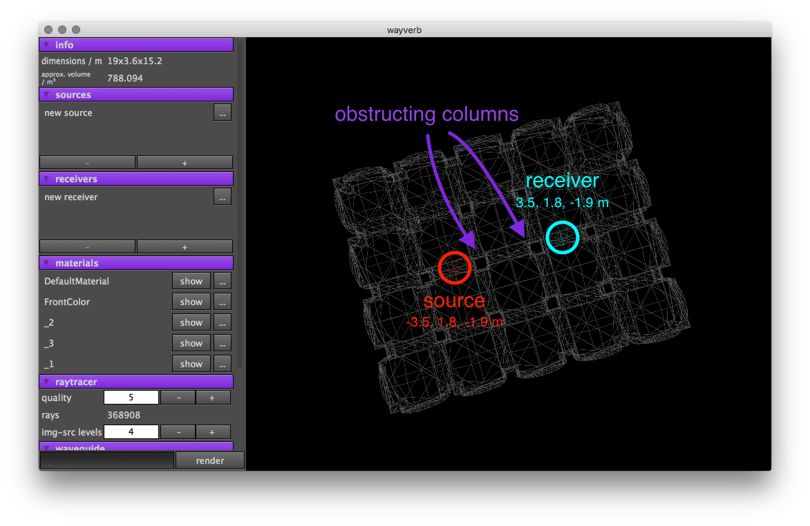
The simulated space is a simple vault-like model, similar to a small hall, but broken up by regularly repeating pillars. The source and receiver are positioned seven metres apart, with their view obstructed by two pillars. If there were no obstruction, a strong direct impulse would be expected after 0.0206 seconds. However, the pillars should block this direct contribution. The model is shown in fig. 7.
In the real world, objects with areas of a similar or greater order to the incident wavelength cause diffraction effects [6, p. 59]. The result of diffraction is that an additional “diffraction wave” is created at the edge of the object, which radiates in all directions. In the vault model, the edges of the pillars should cause diffraction, and in this way, some energy should be scattered from the source to the receiver. This energy will arrive slightly after the direct contribution would have, but before the first early reflection. The shortest possible path from source to receiver which travels around the pillars has a length of 7.12m, corresponding to a time of 0.0209s. Though the image-source and ray tracing models are not capable of modelling diffraction effects, the waveguide model inherently models this phenomenon. Therefore, the impulse response should record a low-frequency excitation at around 0.0209s.

The impulse response graph (fig. 8) shows that low frequency diffraction is in fact recorded. The waveform shows a low-frequency ripple starting at around 0.02 seconds, which occurs before the first impulsive contribution from the geometric models. This is mirrored in the spectrogram, which shows that the low-frequency waveguide contribution (up to 500Hz) has more energy than the geometric contribution at the very beginning of the impulse response. Though the behaviour of the waveguide is physically correct, it highlights the main shortcoming of the hybrid algorithm. For simulations such as this, which rely on the effects of wave phenomena, the physical modelling of the waveguide conflicts with the approximate nature of the geometric algorithms, causing an obvious divide or disconnect between the low and high frequency regions in the output. The impulse response shown here is physically implausible, making it unsuitable for realistic, high-quality reverb effects.
| test | audio file |
|---|---|
| vault |
Late Reflection Details
Having checked the behaviour of early reflections, now the late-reflection performance must be checked. The nature of the ray tracing process means that fine detail (below 1ms precision) is not captured. However, it should be possible to observe reverb features on a larger scale, such as distinct echoes from a long tunnel.
A cuboid with dimensions \(4 \times 7 \times 100\) metres is simulated. The receiver is placed exactly at the centre of the model, with the source positioned two metres away along the z direction. The output should contain a direct contribution at 0.00588s, and some early reflections from the nearby walls. The reverb tail should contain strong echoes every 0.294s, as the initial wave-front reflects back-and-forth between the two end walls.
The tunnel is modelled using absorption coefficients of 0.03 in the bottom five bands, then 0.04, and 0.07 in the highest two bands. The scattering coefficients are set to 0.1 in all bands. This scattering should cause echoes in the reverb tail to be “smeared” in time. To check the effect of the scattering coefficients, the same test is also run using scattering coefficients of 0 in all bands.

The spectrograms show that there are clear increases in recorded energy, occurring approximately every 0.3 seconds after the initial onset. Each echo is followed by its own decay tail. In the case of the non-scattering simulation, the echoes are clearly separated, with very short tails. When the scattering is increased, the tails become longer, and the individual echoes become less defined. This is expected: when there is no scattering, rays travelling in any direction other than along the length of the tunnel will bounce between the walls many times, attenuated each time. These contributions may arrive at any time at the receiver, however, their amplitude will be greatly reduced. The rays travelling directly between the ends of the tunnel will be reflected fewer times, will lose less energy, and will produce louder regular contributions. When scattering is introduced, the ray paths are less regular, giving less correlation between the number of reflections and the time at which the ray is recorded. This in turn leads to a more even distribution of recorded energy over time.
| test | audio file |
|---|---|
| tunnel with scattering | |
| tunnel without scattering |
Directional Contributions
To test that microphone modelling behaves as expected, two cardioid microphones are placed in the exact centre of the “large” cuboid room, facing towards and away from the source, which is positioned at a distance of 3m along the z-axis.
An ideal cardioid microphone has unity gain in its forward direction, and completely rejects waves incident from behind. In this test, the direct contribution from the source originates directly in front of one receiver and behind the other, so it should be present only in the signal measured at the capsule facing the source. The next-shortest path from the source to the receivers is caused by reflections from the floor and ceiling, both with path lengths of 5m, corresponding to 0.0147s. These paths should cause a strong contribution in the capsule facing the source, and a quieter contribution in the capsule facing away. There is a path with a length of 11m which should strike the receivers from the opposite direction to the source. At this time, there should be a large contribution in the away-facing capsule, and a small contribution in the towards-facing capsule.
These expectations are reflected in the results, shown in fig. 10. The impulse response is silent in the away-facing capsule at the time of the direct contribution, 0.00882s. The first significant level is recorded at 0.0147s, with a loud contribution seen at 0.0324s. In the capsule facing towards the source, the first two contributions are loud, with no contribution at 0.0324s. These results are consistent across the spectrum, indicating that the microphone model is matched between both simulation methods.

| test | audio file |
|---|---|
| cardioid mic facing away |
Binaural Modelling
Finally, the binaural model is tested. A concert hall measuring approximately \(33 \times 15 \times 50\) metres is simulated (shown in fig. 11), with wall absorptions increasing from 0.25 in the lowest band to 0.67 in the highest band, and scattering at 0.1 in all bands. The source is placed in the centre of the stage area, and the receiver is placed 10m along both the x- and z-axes relative to the source. The receiver is oriented so that it is facing directly down the z axis, meaning that the source is 14.1m away, on the left of the receiver.

The simulation produces output impulse responses for both the left and right ears. All of Wayverb’s simulation methods (image-source, ray-tracing and waveguide) use HRTF data to produce stereo effects based on interaural level difference. The image-source method additionally offsets the receiver position to produce interaural time difference effects, so in the outputs, slight time differences in the early reflections between channels are expected, and small level differences should be seen throughout both files.
In particular, the direct contribution would normally arrive at 14.1/340=0.0416s. However, the left “ear” is actually slightly closer to the source, and the right ear is slightly further away, which means that the first contribution should be at 0.0414s in the left channel, and 0.0418s in the right. The right ear is obstructed by the listener’s head, and should therefore have a reduced level relative to the left ear.
The expected behaviour is observed in the outputs, which are shown in fig. 12. The earliest contribution in the left channel occurs at 0.0414s, and has a greater level than the right channel’s contribution at 0.148s. The left-channel early reflections have an overall higher level than the early reflections in the right channel. However, as the impulse response progresses and becomes more diffuse, the energy levels equalise between channels.

| test | audio file |
|---|---|
| binaural receiver, source left |
Summary
A simulation program, Wayverb, has been implemented and its feature set described. Tests have been run to gauge how closely Wayverb’s simulation matches predicted behaviour. These tests have been designed in accordance with the primary research goal, which was physical plausibility. The results show that changes in parameters cause appropriate changes in the outputs:
- Larger rooms have longer reverb times than smaller rooms.
- Rooms with high absorption produce shorter reverb times than more reflective rooms.
- When the source and receiver are moved apart, the ratio of direct to reverberant sound decreases.
- Obstructions in the room cause diffraction.
- Long reflective rooms produce distinct echoes.
- Receiver modelling produces appropriate direction-dependent attenuation.
The main downfall of Wayverb’s simulation method is an obvious mismatch between the low- and high-frequency regions of the output. The room-size and absorption tests showed that reverb times above and below the model crossover frequency differ by significantly more than the JND. Also, the simulation as a whole is not accurate: in the largest room, the broadband reverb time differed from the Sabine prediction by more than the JND. Although the effects of changing parameters are plausible, the overall simulation results are not.
Tests have not been presented regarding the two lesser research goals of efficiency and accessibility. Ideally, benchmarks and usability tests would have been conducted. The shortcomings of the test procedure, and the implications thereof, are analysed in the following chapter.
References
[1] “Assimp Supported Formats.” 2017 [Online]. Available: http://www.assimp.org/main_features_formats.html. [Accessed: 13-Jan-2017]
[2] “Room EQ Wizard Room Acoustics Software.” 2017 [Online]. Available: https://www.roomeqwizard.com/. [Accessed: 12-Jan-2017]
[3] “Operatic Voice The Open Acoustic Impulse Response Library.” 2017 [Online]. Available: http://www.openairlib.net/anechoicdb/content/operatic-voice. [Accessed: 16-Jan-2017]
[4] International Organization for Standardization, Geneva, Switzerland, “ISO 3382-1:2009 acoustics – measurement of room acoustic parameters – part 1: Performance spaces.” 2009.
[5] M. Hodgson, “When is diffuse-field theory accurate?” Canadian Acoustics, vol. 22, no. 3, pp. 41–42, 1994.
[6] H. Kuttruff, Room Acoustics, Fifth Edition. CRC Press, 2009.